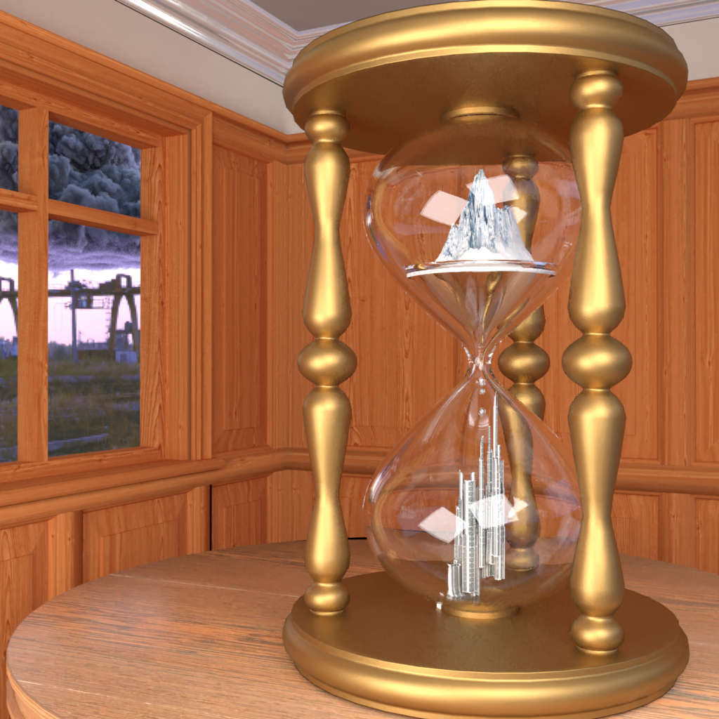
 Xiaohongshu - Hourglass, Bangbing Pan
# Qi Ma
ID | Short Name |Points | Features (if required) & Comments
--------|---------------------------|-------|------------------------------------
5.10.2 | Simple Extra Emitters | 5 | directional light
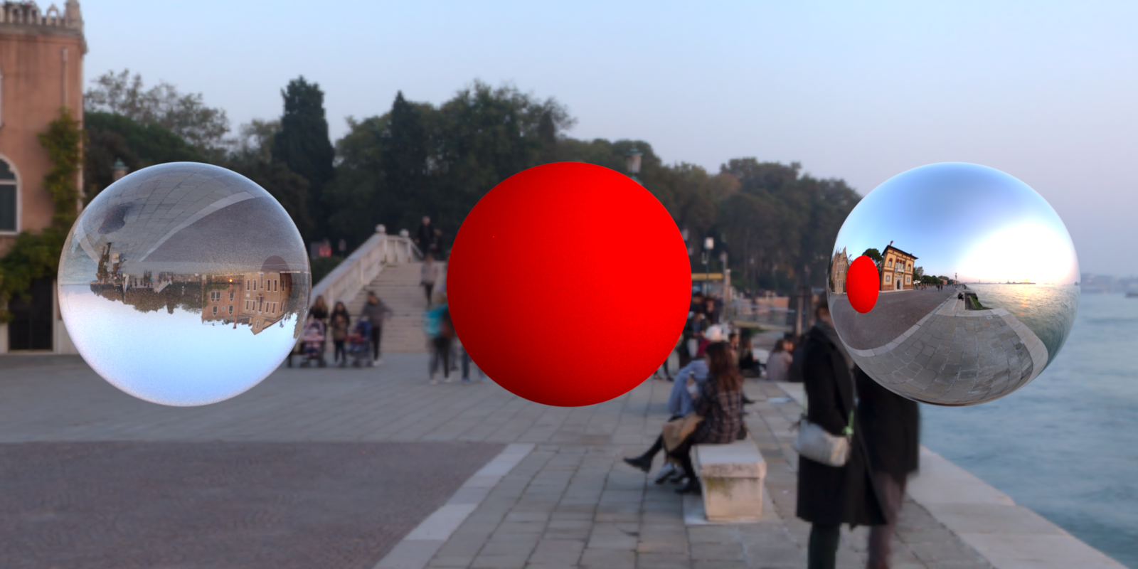
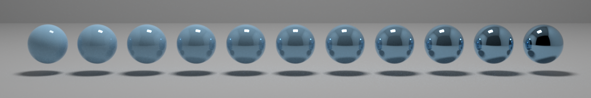
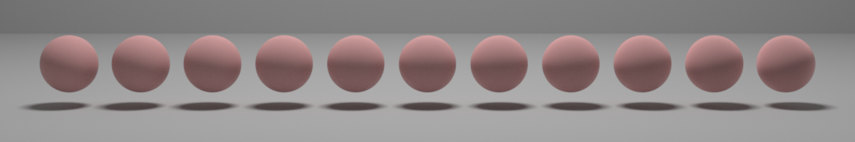
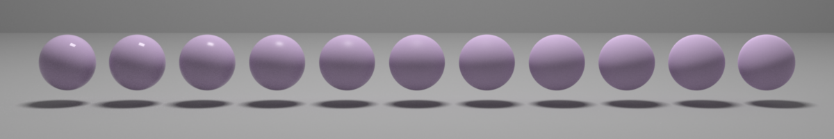
5.16.1 | Anisotropic Phase Function | 5 | Henyey-Greenstein
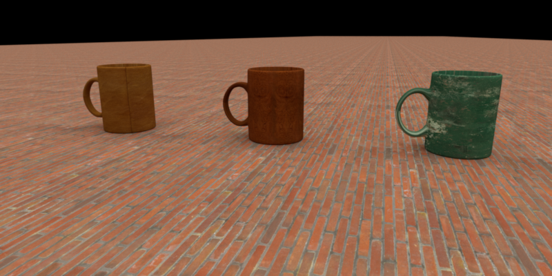
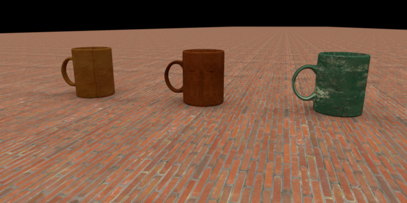
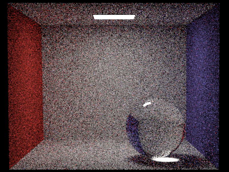
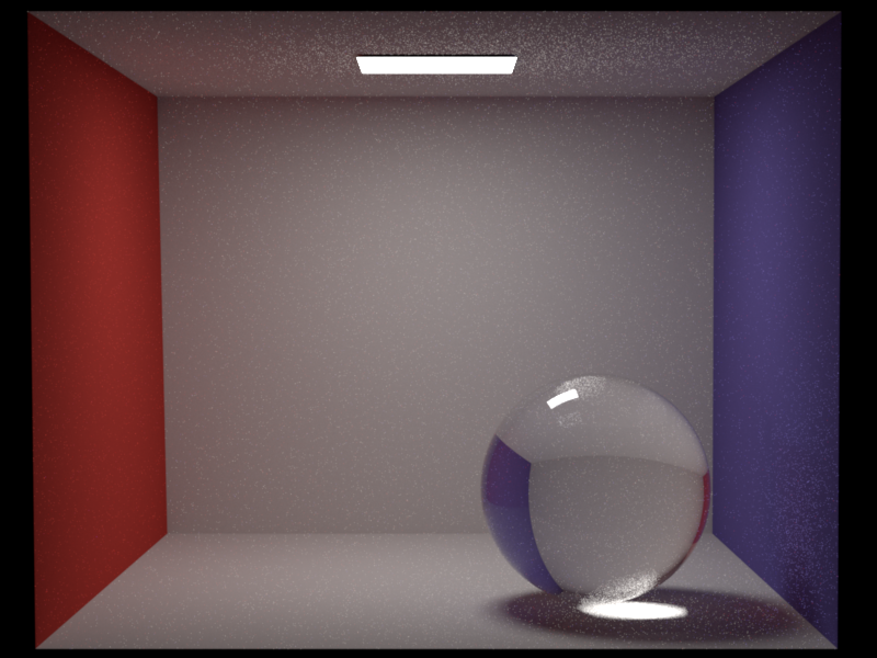
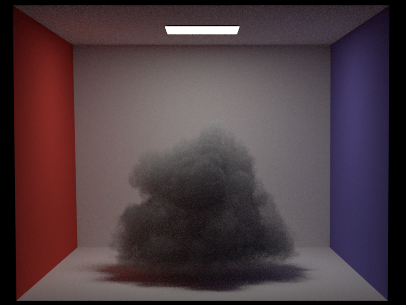
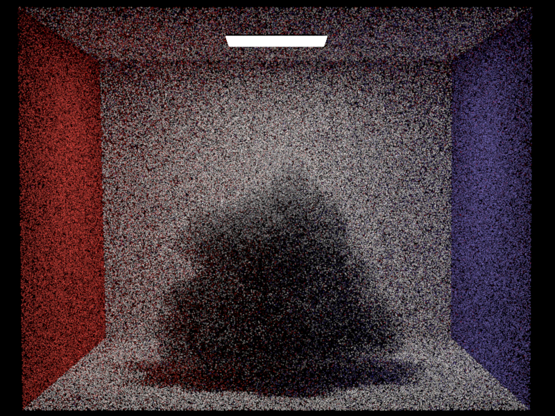
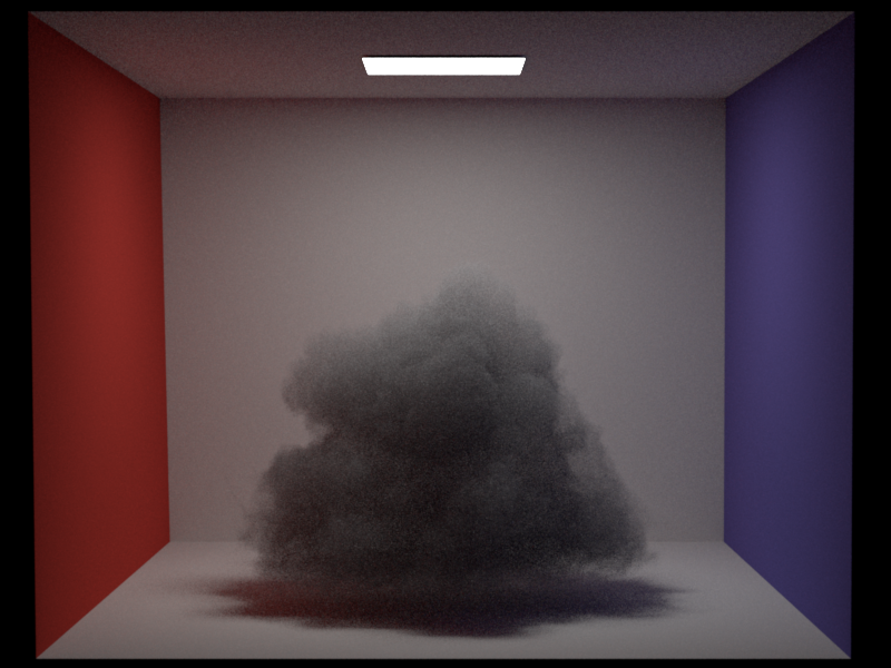
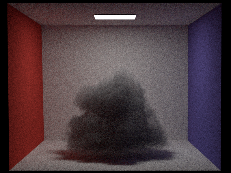
10.3 | Simple Denoising | 10 |
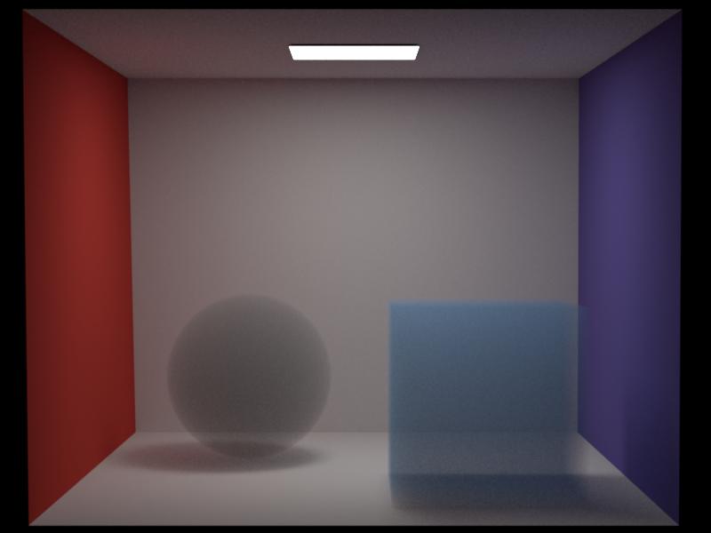
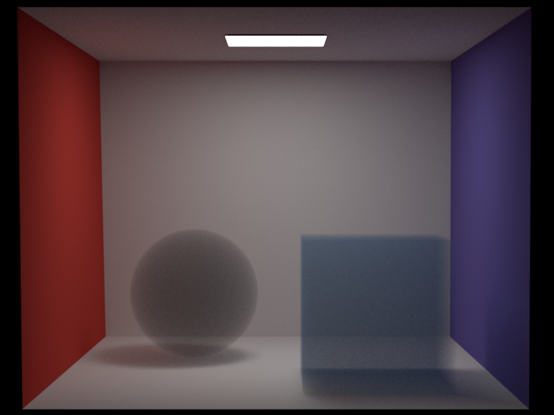
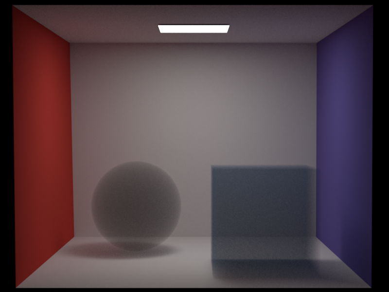
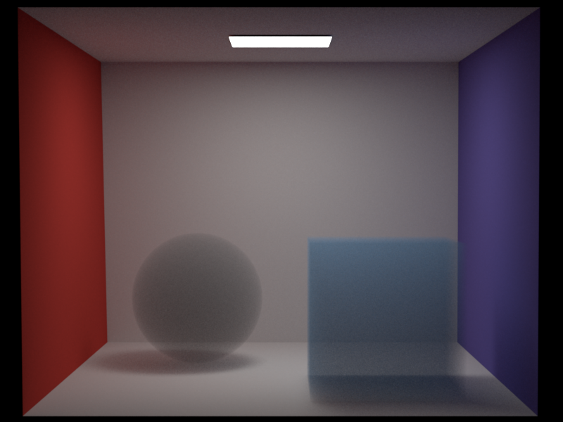
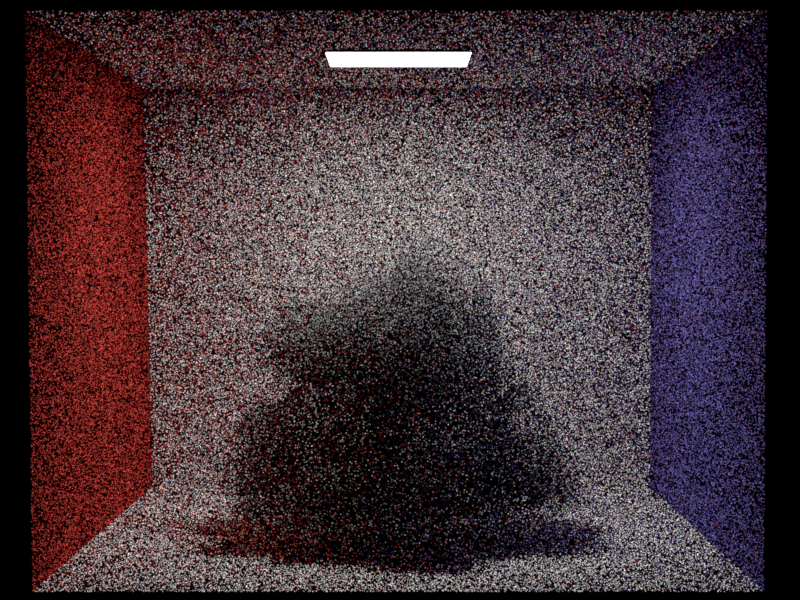
10.9 | Different distance sampling and transmittance estimation methods: ray marching, delta tracking and ratio tracking | 10 |
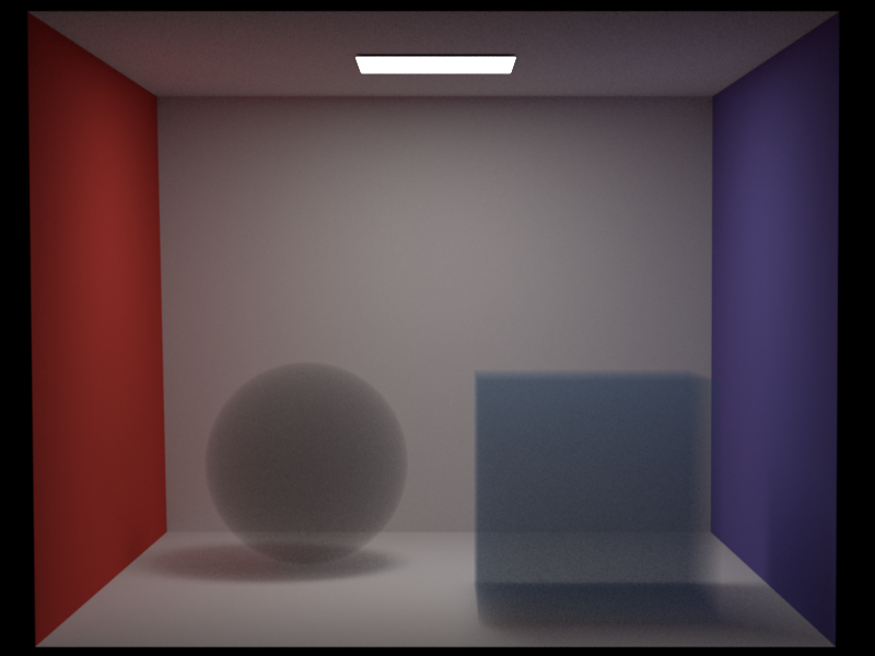
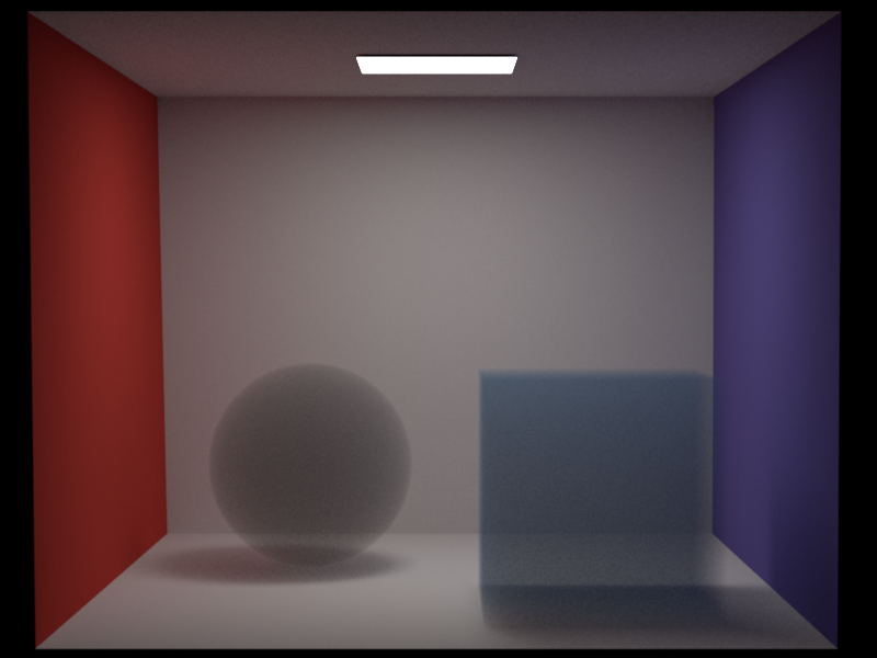
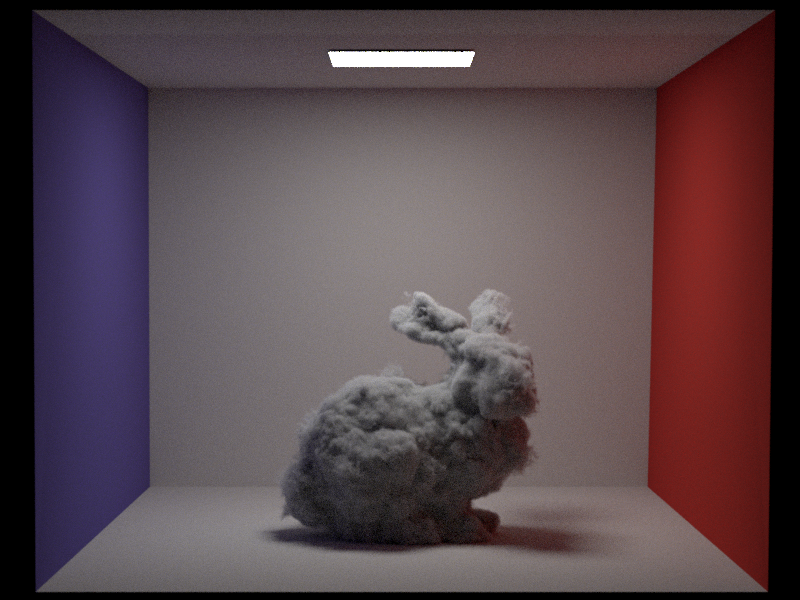
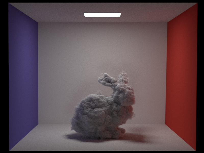
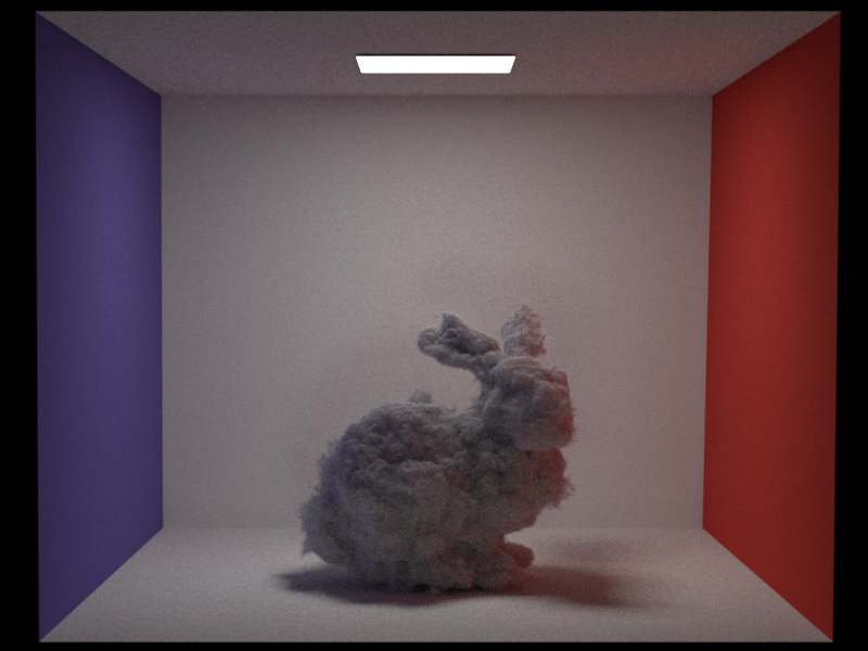
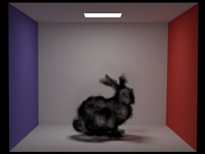
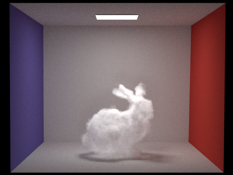
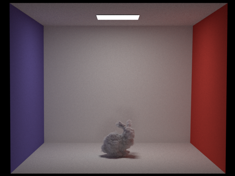
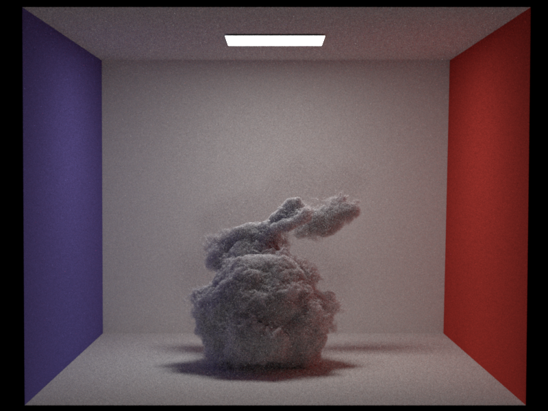
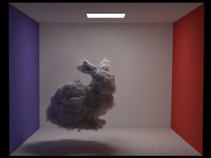
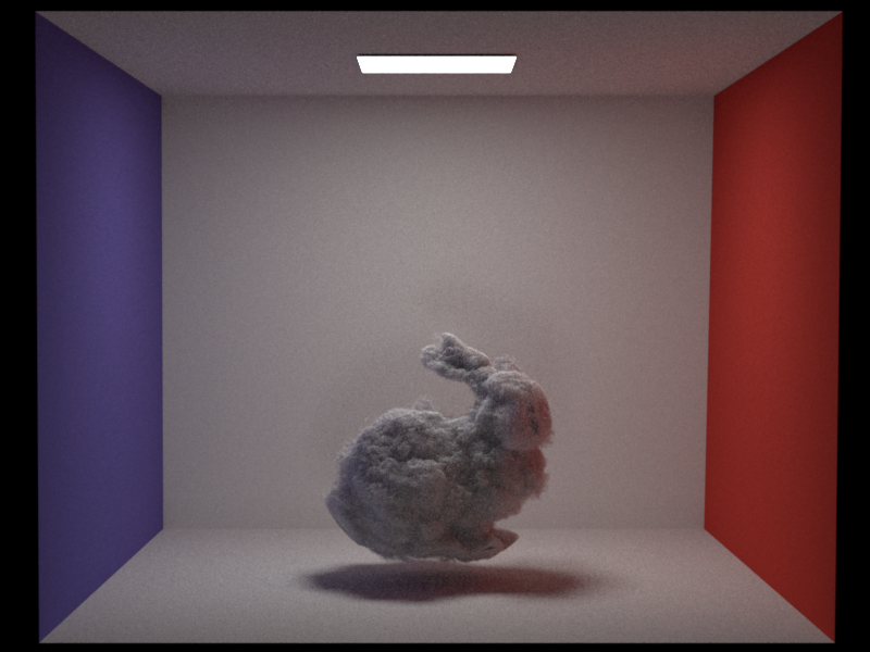
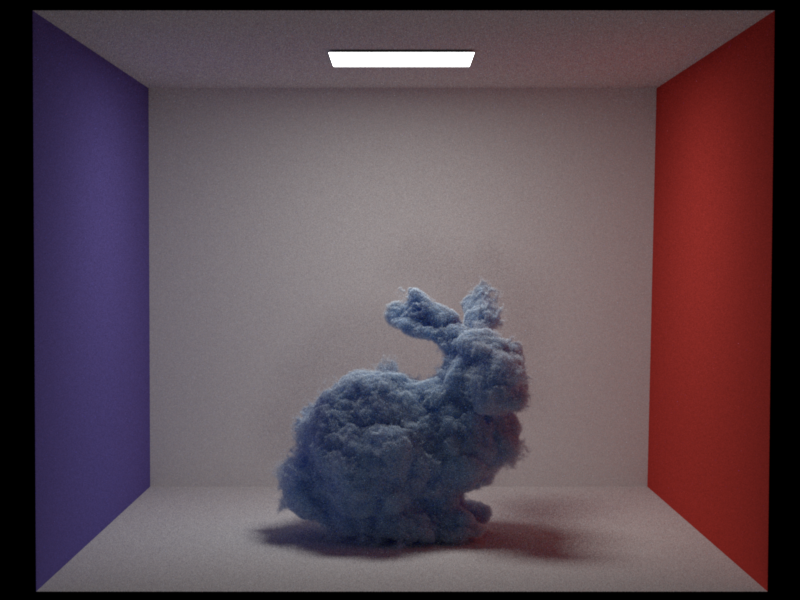
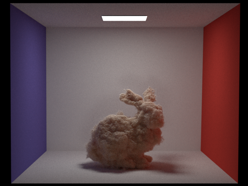
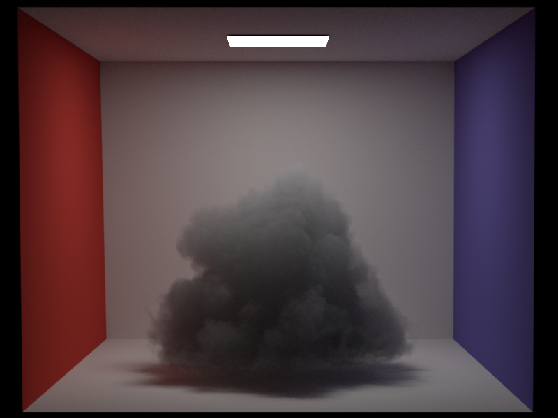
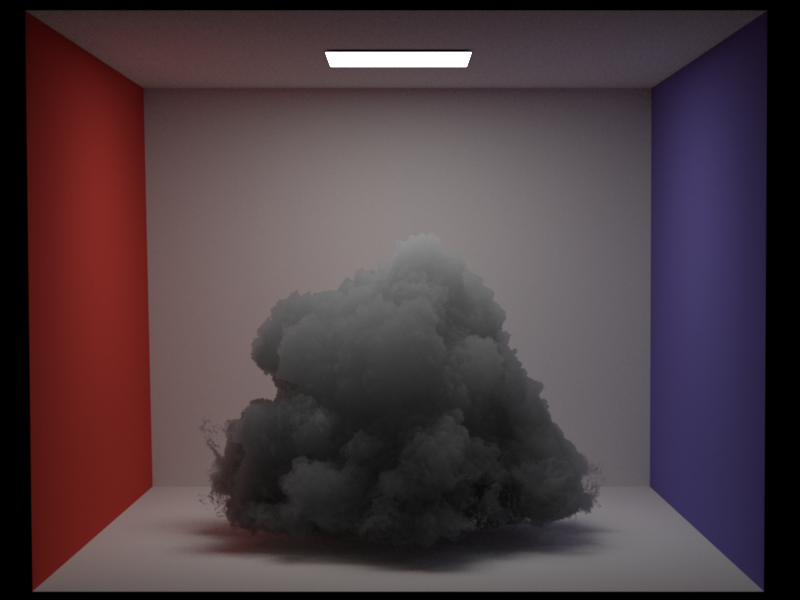
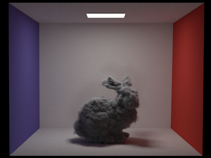
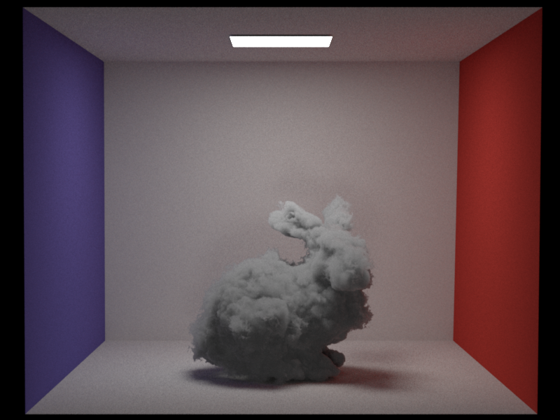
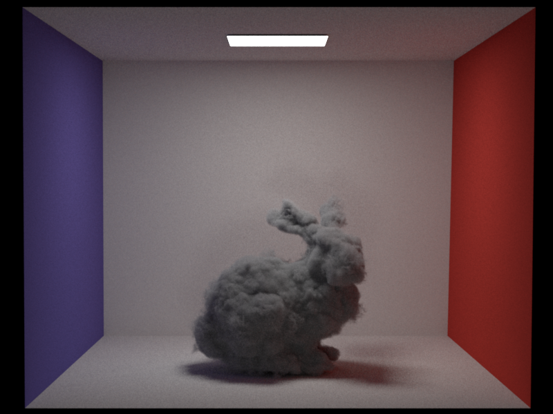
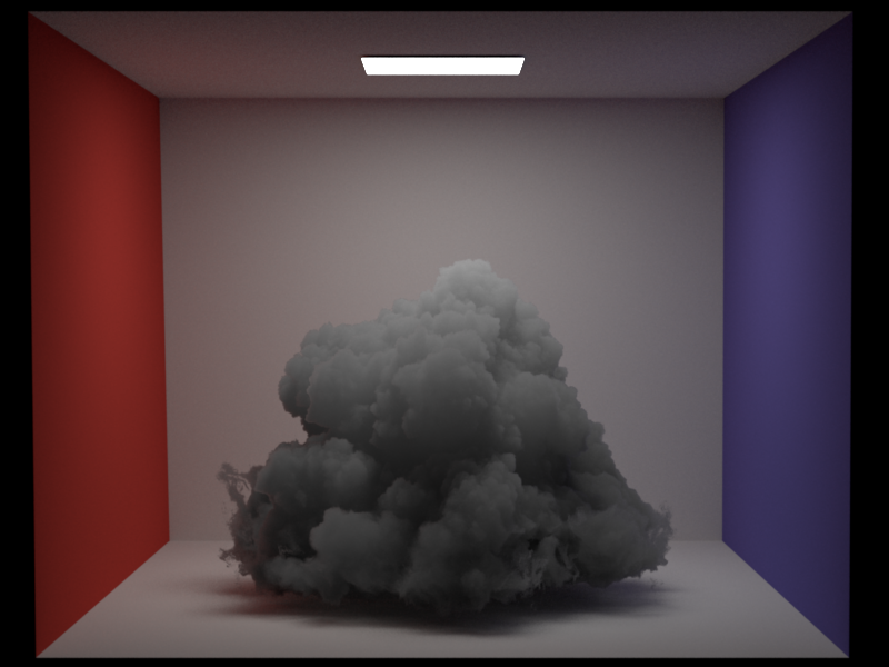
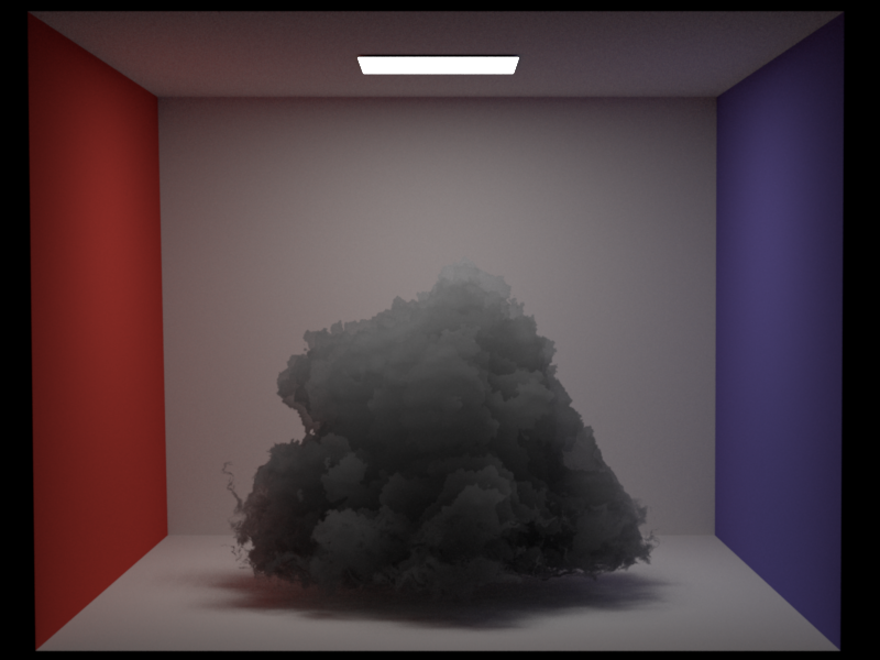
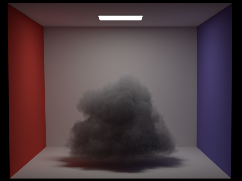
30.1 | Heterogeneous Participating Media | 30 |
Total || 60 |
## Simple Extra Emitters: Directional Light (5 Points)
### Updated Files
- `include/nori/emitter.h`
- `src/directional.cpp`
- `src/path_mats.cpp`
- `src/path_mis.h`
- `src/vol_path_mis.cpp`
### Implementation
Directional light is a type of light source that emits light in a specific direction with uniform intensity that does not attenuate over distance.
For the implementation of the directional light, we created a new class `DirectionalEmitter` in the `directional.cpp` file.
The `DirectionalEmitter` class inherits from the `Emitter` class and includes properties for the light's intensity and direction.
The core functionality is in the `sample` method, which calculates the projection of the distance from the reference point to the light source projection center onto the light source direction.
The light source projection center is estimated from the world center and world radius based on the scene or be specified in the scene xml file.
It also sets up a shadow ray for visibility testing and assigns values to key fields in the `EmitterQueryRecord`, including the light position, direction, and normal.
The `eval` and `pdf` methods return fixed values (`0` and `1`, respectively), reflecting the delta nature of the light source.
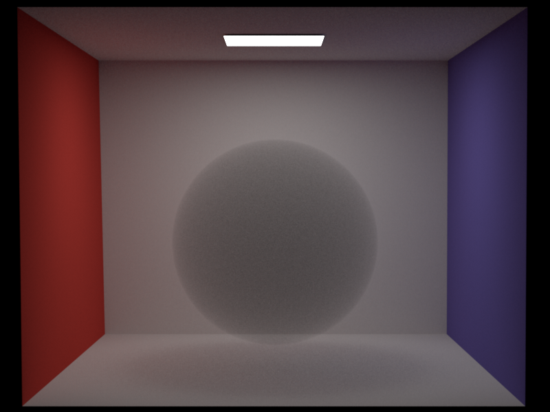
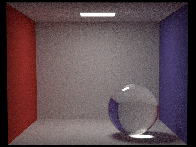
### Validation
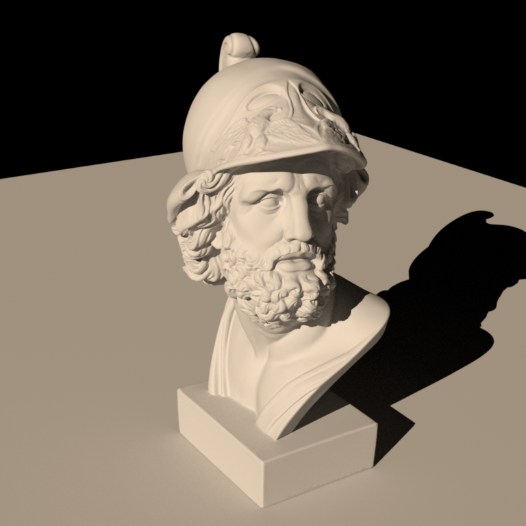
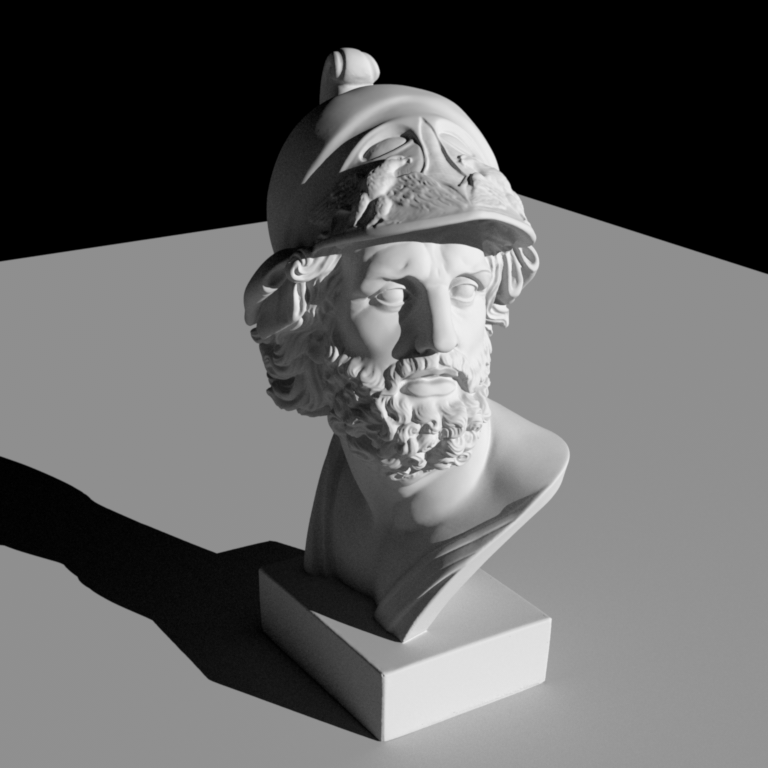
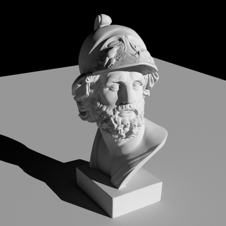
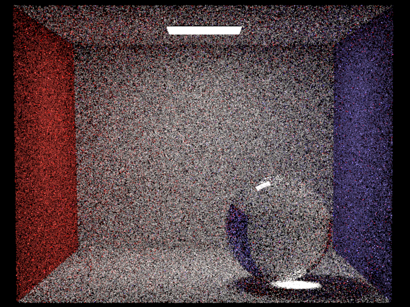
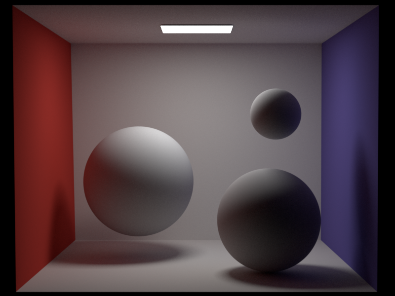
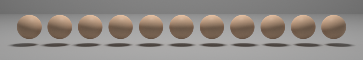
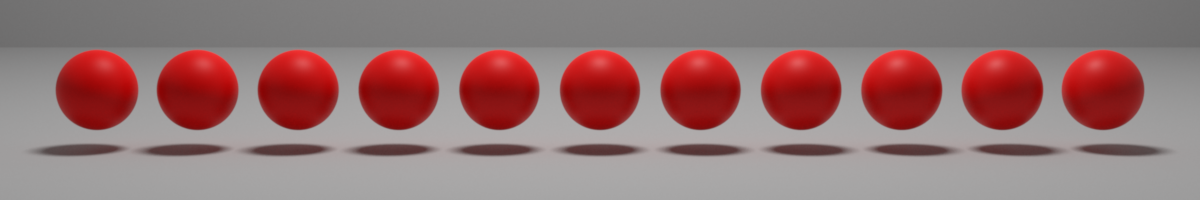
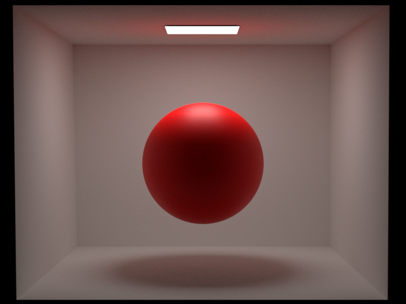
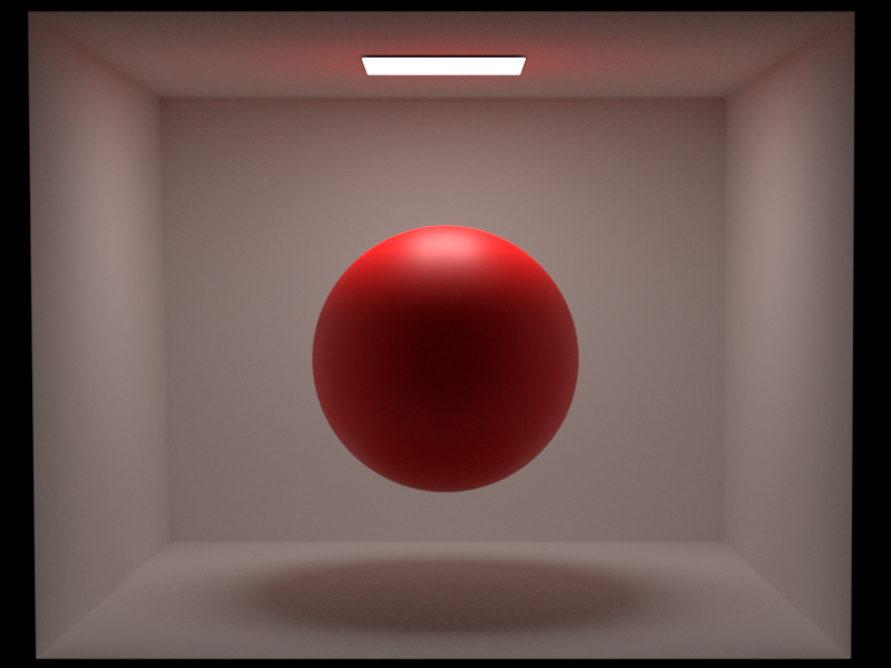
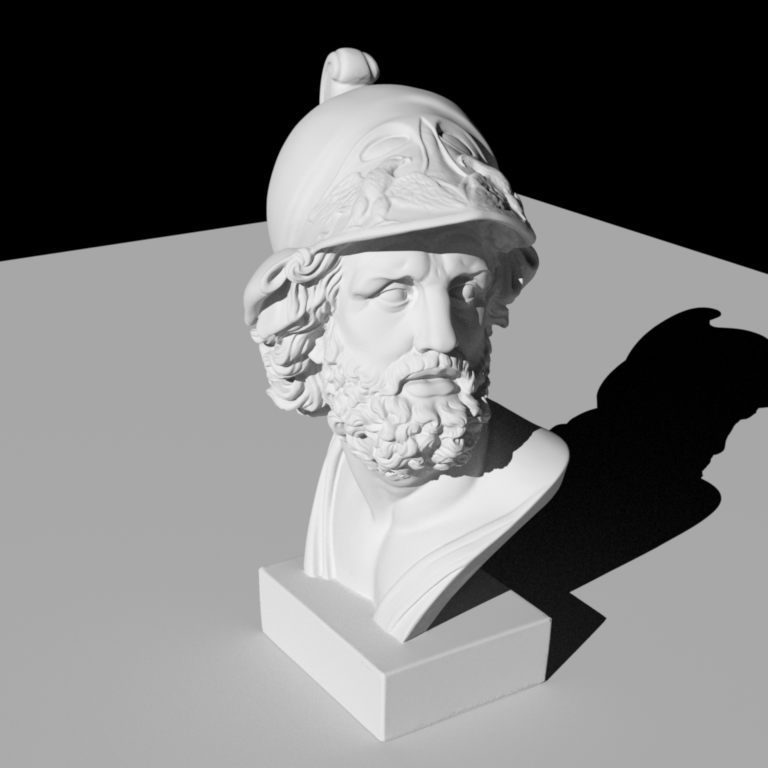
We compared the directional light with the same functionality in Mitsuba. The direction of the light and its radiance were adjusted to validate the correctness of the implementation.
#### Comparison 1: Uniform Intensity
- Intensity: `(5, 5, 5)`
- Direction: `(0.401387, -0.444440, -0.800851)`
- Samples Per Pixel (SPP): 256
Xiaohongshu - Hourglass, Bangbing Pan
# Qi Ma
ID | Short Name |Points | Features (if required) & Comments
--------|---------------------------|-------|------------------------------------
5.10.2 | Simple Extra Emitters | 5 | directional light
5.16.1 | Anisotropic Phase Function | 5 | Henyey-Greenstein
10.3 | Simple Denoising | 10 |
10.9 | Different distance sampling and transmittance estimation methods: ray marching, delta tracking and ratio tracking | 10 |
30.1 | Heterogeneous Participating Media | 30 |
Total || 60 |
## Simple Extra Emitters: Directional Light (5 Points)
### Updated Files
- `include/nori/emitter.h`
- `src/directional.cpp`
- `src/path_mats.cpp`
- `src/path_mis.h`
- `src/vol_path_mis.cpp`
### Implementation
Directional light is a type of light source that emits light in a specific direction with uniform intensity that does not attenuate over distance.
For the implementation of the directional light, we created a new class `DirectionalEmitter` in the `directional.cpp` file.
The `DirectionalEmitter` class inherits from the `Emitter` class and includes properties for the light's intensity and direction.
The core functionality is in the `sample` method, which calculates the projection of the distance from the reference point to the light source projection center onto the light source direction.
The light source projection center is estimated from the world center and world radius based on the scene or be specified in the scene xml file.
It also sets up a shadow ray for visibility testing and assigns values to key fields in the `EmitterQueryRecord`, including the light position, direction, and normal.
The `eval` and `pdf` methods return fixed values (`0` and `1`, respectively), reflecting the delta nature of the light source.
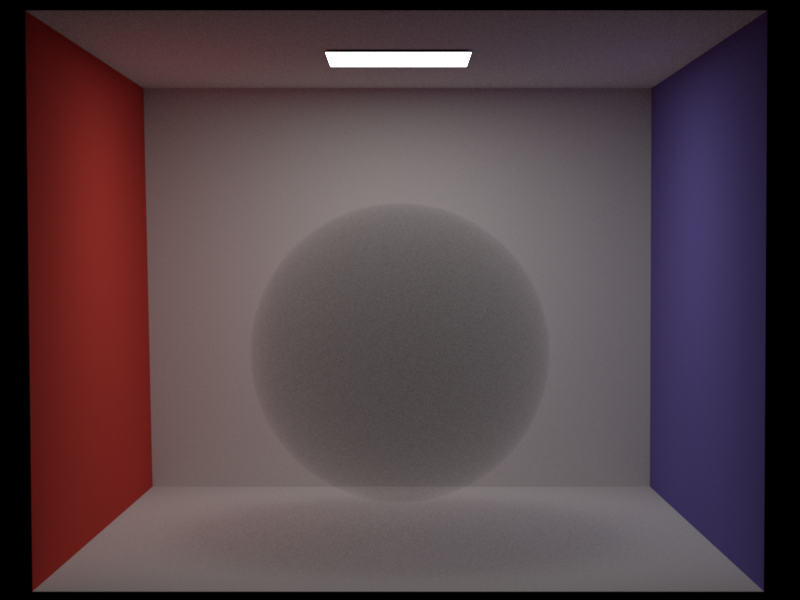
### Validation
We compared the directional light with the same functionality in Mitsuba. The direction of the light and its radiance were adjusted to validate the correctness of the implementation.
#### Comparison 1: Uniform Intensity
- Intensity: `(5, 5, 5)`
- Direction: `(0.401387, -0.444440, -0.800851)`
- Samples Per Pixel (SPP): 256